Gini

Blog | Turning Gini into Profits

Written by Rodrigo Sanabria, Director Partner Success, Latin America

On a prior post by Carlos del Carpio (“The Economics of Credit Scoring”), we discussed the business considerations to assess the merit of a risk model. In this post, I will address how a good origination model impacts the bottom line of a company’s P&L.

These principles may be adapted to look into other types of models used at later stages of a loan life, but on this post we will only address loan origination.

From a business point of view, an origination model is a tool that helps us aim at the “sweet spot”: where we maximize profits. A simple way to think about it is as a trade-off between the cost of acquisition (per loan disbursed) and cost of defaults (provisions, write-offs): The higher the approval rate, the lower the cost of acquisition, but the number of defaults go up.

How do we go about finding the sweet spot? I’ll try to explain it below.

Figure 1

Figure 1

A good model has a good Gini. A “USEFUL” model creates a steep probability of default (also known as PD) curve – we usually refer to it as a “risk split”.


Figure 1 shows the performance of a model based on psychometric information used by an MFI. The Gini (not shown in the graphic) is pretty good (0.28). The risk split is great: the people in the lower 20% of the score ranking are about 9 times more likely to default than those in the top 20%.


Knowing the probability of default for a given group, we may set a credit policy. Basically, we need to answer: “what would the default look like given an acceptance rate?”
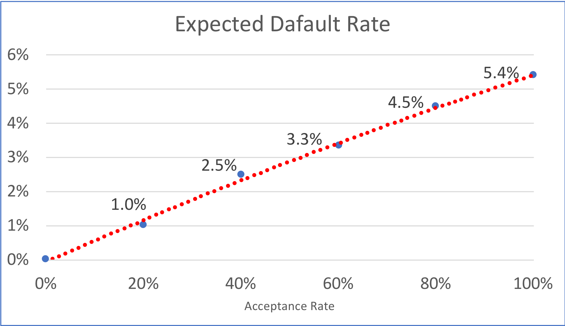
 

Figure 2

Figure 2


We have re-plotted the same data in Figure 2, but now we express the probability of default in accumulated terms. Basically, the graph shows that if we were to accept 80% of this population sample, we would have a 4.5% PD, but if we were to accept 40%, the PD would go down 2 points to 2.5%.

Now, from a business point of view, we still do not have enough information to decide. Do we?


Where would the profit be maximized?

The total cost of customer acquisition is mainly fixed. Whatever we spend on marketing and sales to attract this population, will not change if we reject more or fewer applicants. So, the cost per loan disbursed would grow as we reduce the acceptance rate.

Of course, the higher the acceptance rate, the larger the portfolio, and the more interest revenue we get. BUT, the higher the provisions and write-offs. The combination of these 2 variables (cost of acquisition and net interest income) produces an inverted U-shaped curve that uncovers the “sweet spot”

Figure 3

Figure 3

The current credit policy is yielding a profit at 100% acceptance rate (see Figure 3) because the sample being analyzed corresponds to all the customers that were accepted (i.e. we have repayment data about them). So, the portfolio is profitable.

But the sweet spot seems to be shy of 60% acceptance rate. If this FI were to cut down its approval rate to that level, profits would increase by about a third, and its return on portfolio value would almost double. Of course, there are other considerations around market share and capital adequacy that may play a role in such a strategic decision, but the opportunity is clearly uncovered by the model.


In my experience, the sweet spot usually lies within 30%-70% acceptance rates, driven by marketing expenditures, interest rates, cost of capital, sales channels, and regulation.

What if the shape of the curve shows a continuous positive growth? The sweet spot is at a 100% acceptance rate! – have we reached risk karma? – Most likely, the answer is no (but almost!).
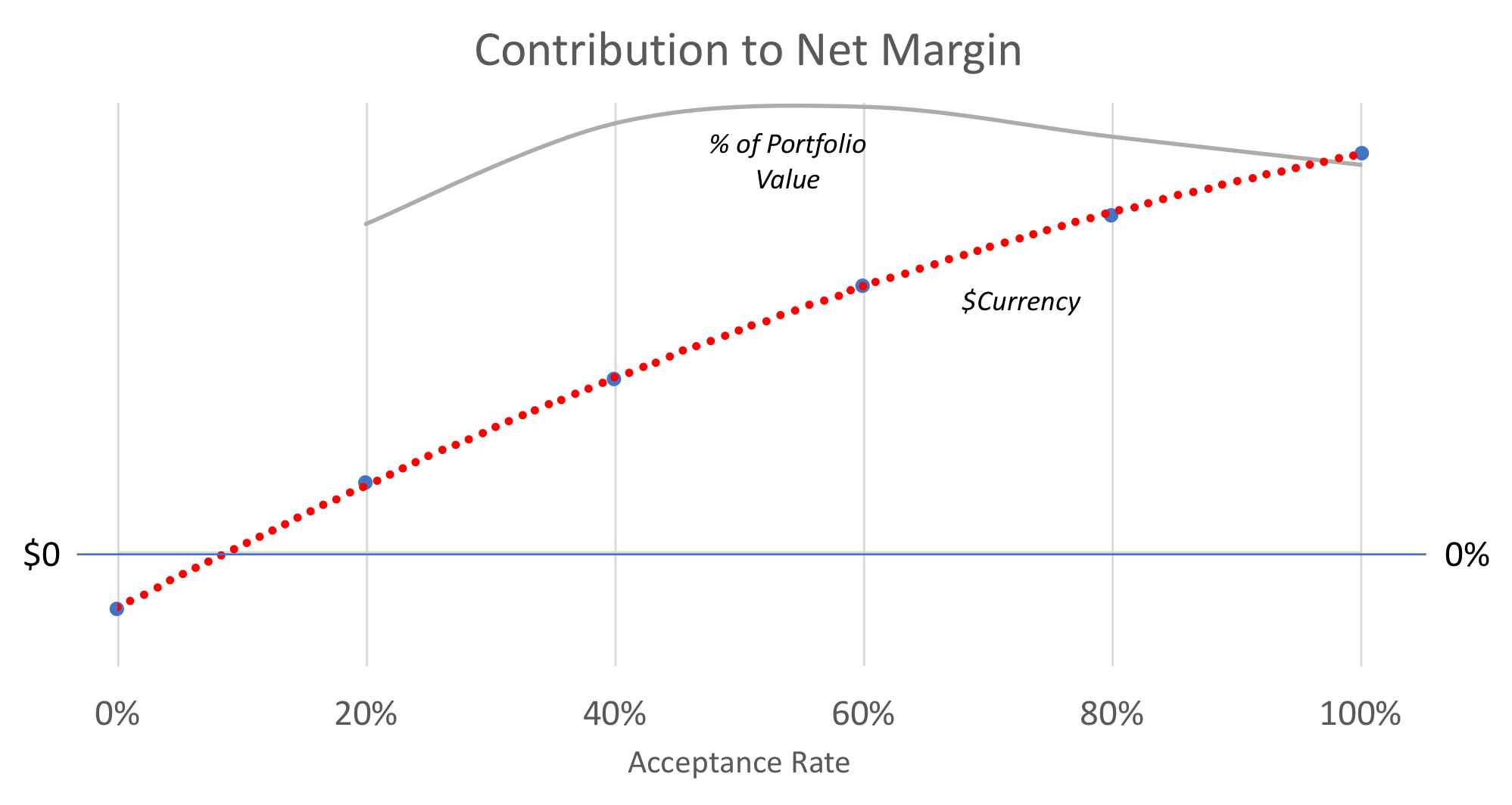
Figure 4

Figure 4

Most likely, we are leaving money on the table. Some business rule may be filtering people before they are scored. I have experienced this situation while working with lenders. For example, a traditional bank was filtering out all SMEs that had been operating for less than X years. This bias in the population was creating a great portfolio from a PD point of view, but there was clearly an opportunity to include younger businesses. As you can see in Figure 4, the maximum return on the portfolio was achieved at 60% approval rate, but they could increase profits by approving beyond the current acceptance rate. Depending on their cost of capital, it may be a good idea to expand the portfolio by approving more people.

In summary, think of your origination model as a business tool. Don’t stop at looking at Gini to assess a model’s merit. Understand how your profitability would be impacted by changes in your acceptance rate. If the PD curve is steep enough, you may capture quite a lot of value by applying the model to either reduce or increase your acceptance rate.

Blog | On the use (and misuse) of Gini Coefficients in Credit Scoring: the Economics of Credit Scoring

This is the fourth part of a series of blog posts about Ginis in Credit Scoring. See also part 1, part 2, part 3.
image4.png

Gini Coefficients and the Economics of Credit Scoring

On a global scale, billions of dollars in debt are granted every year using decisions derived from credit scoring systems. Financial institutions critically depend on these quantitative decision to enable accurate risk assessments for their lending business. In this sense, as with any tool that serves a business purpose, the application of credit scoring is not ultimately measured by its statistical properties, but by its impact in business results: how much can Credit Scoring help to increase the benefit and/or to decrease the cost of the lending business.

Assessing Credit Scoring from a business perspective could sound pretty obvious. However, given the typical compartmentalization of roles that could exist at lending institutions, where Risk and Modeling teams can be completely separated from Commercial departments, it could be easy sometimes to focus too much on the statistical aspects of credit scoring such as Ginis, and forget the ultimate business nature of its purpose. Although there is a clear positive relationship between economic benefits and predictive power, there are also certain elements that can affect the balance between costs and benefits. In this post, we discuss some of these elements and explain their role in the cost-benefit analysis of credit scoring.


The benefits of credit scoring

The benefit of credit scoring derives from its ability to accurately identify good customers, and discriminate them from bad customers. The more good customers a model can identify, the greater the interest income that can be generated from a credit portfolio. And the more bad customers it can discriminate, the lower the losses for the credit portfolio. In this sense, the economic benefit of credit scoring can be amplified by two things: the volume of customers, and the size of the credit disbursed to these customers.

Take for example the portfolio of microfinance institution “A” with several thousands of customers but very small loan amounts, and compare it against a smaller microfinance institution “B” providing loans of the same size to a portfolio of just a few hundred customers. Both institutions can see a similar increase of 1% in the predictive power of their credit scoring models, however, the increase in economic benefit yielded from this increase in predictive power will be different just because of the different sizes of portfolio volumes. Everything else being equal, the higher the volume of the portfolio, the higher the potential economic benefit of credit scoring.

The same can be argued for the size of credit disbursed to the customers of a portfolio. For example, take an SME lending institution with just a few thousands of customers but with relatively high credit amounts in the hundreds of thousands of dollars. An increase of 1% in predictive power could bring just a handful of new good clients into the portfolio, or avoid the disbursement of a handful of very bad loans. However a change in just a handful of good or bad clients can be enough to generate a considerable increase of economic benefit in the portfolio given the large size of the loans.


The costs of credit scoring

The costs of Credit Scoring can be split in two parts. First, the cost of developing a new model, and secondly, the cost of implementing and maintaining credit scoring models.

If we assume lending institutions are at a stage of technological maturity in which all the necessary data to create a credit scoring model exists and is continuously updated with certain level of quality and integrity, then the first type of cost just depends on the complexity of the modeling process. The whole process of building a model includes data extraction and cleaning, feature engineering, feature selection and the selection of a classification algorithm.

Depending on the lending institution, this process can be handled by a single data scientist (e.g. think of the CRO of a small Fintech startup), or it can be handled by a large department including many different teams with different roles such as data engineers, data scientists and software engineers (e.g. think of a large multinational bank). At the same time, the teams in charge of the model building process can be comprised of junior analysts fresh out of college using well-known standard techniques or include teams of PhDs in computer science doing advanced machine learning. At the end, the cost involved in developing the credit scoring models will depend on how much complexity and sophistication can be afforded and/or needs to be put into the process.

Once the model has been built, it also needs to be implemented and monitored over time. The costs involved are not trivial. Again, they will depend on the stage of technological maturity of the financial institution and the complexity and sophistication required. For example, in some cases the implementation of a credit scoring model can be as simple as creating an Excel calculator loaded with the coefficients of a logistic regressions where some values are manually inputted by a Loan Officer to get a score (e.g. think of a small MFI in the rural area of a developing country). Or it can be as complex as a Python package in a cloud-hosted decision engine integrated in the online platform of a large bank. The handling of big data, software development and testing, as well as the security and legal aspects involved in the deployment of a credit scoring system can considerably increase its costs. And all this, without even considering if the teams that will monitor the performance of the models implemented on a defined frequency basis are dedicated full time, or they are just the same team that also did the modeling and/or deployment.


Bottom-line:  The statistical classification accuracy measured by Gini coefficients are indicative of some part of the benefits of using credit scores, but they are not the most important nor the final metric when assessing the cost-benefit of credit scoring. The reason is because the benefits of credit scoring can be influenced by the volumes of customers and the size of the credit. And the costs of credit scoring ultimately depends on the stage of technological maturity of the lending institution, as well as how much complexity and sophistication can be afforded and need to be put in the development, deployment and monitoring of credit scoring models.   

So next time you need to make a decision about using Credit Scores to boost your lending business, ask how much they can help to increase the benefits of the business, and how much they can help to decrease its cost. The final decision will depend on a lot more than just Ginis.


At LenddoEFL, we have the expertise to help you boost the benefits and reduce the costs of credit scoring using traditional and alternative data. Contact us for more information here: https://include1billion.com/contact/.


Blog | On the use (and misuse) of Gini Coefficients in Credit Scoring: Gini and Acceptance Rate

photo-1506704810770-7e9bbab1094b.jpeg

This is part 3 in a series of blog posts about Ginis in Credit Scoring. Read part 1 and part 2.

The relationship between Gini Coefficients and Acceptance Rate

One of the most frequent uses of Credit Scores is to decide whether to admit or reject an applicant applying for loan. This is usually called an “Admission score” or “Origination score”. A key decision around this use case is the selection of a score cut-off that will determine a threshold for admission. This cut-off value determines the acceptance rate of the population.

If the score is working well and predictive power is good, the relationship between acceptance rate and default rate will be positive. The higher the acceptance rate, the higher the default rate of the accepted population and vice versa. The direction of this relationship also has two implications: when acceptance rate is higher, the absolute number of bad loans (i.e. non-performing loans) or “bads” will also be higher, and the proportion of these “bads” in respect to the total loans in the accepted population will be higher too.


What does this mean in practical terms?

It means that the predictive power as measured by a Gini coefficient for the exact same score at different levels of acceptance rate for the exact same population will be different. The higher the acceptance rate, the higher the Gini coefficient and vice versa.

This is something that can be easily tested. If you have a portfolio and a score with good predictive power, you can calculate the Gini coefficient for different score cutoffs or acceptance thresholds and the results should look something similar to this example of a typical credit portfolio:

image6.png

So for example, if there is a change in credit policy and the acceptance rate is lowered from 60% to 40%, the Gini coefficient for the same score over the new sample may also be lower. Does that mean the model is not working anymore? Absolutely not. All the contrary, it’s probably just a good signal that the score is doing a good job. Once a change in acceptance rate is implemented, results should be assessed by the change in default rate, not in predictive power.

Bottom-line:  To judge the predictive power of a Credit Score by the means of Gini, you also need to take into account the Acceptance Rate at which the Gini coefficient is measured. Lower Acceptance Rates will tend to have lower Gini coefficients by construction, even if it is the same exact score over the same population.

The fundamental reason behind this phenomenon was discussed in the part 2, where we explained why Gini coefficients should only be directly compared over the exact same data samples, even if the two samples correspond to the same population.


By: Carlos Del Carpio, Director of Risk and Analytics, LenddoEFL

By: Carlos Del Carpio, Director of Risk and Analytics, LenddoEFL